Updated
• 7 min read (EN)
Gordon Growth Formula: Fair Value and g = Retention × ROE
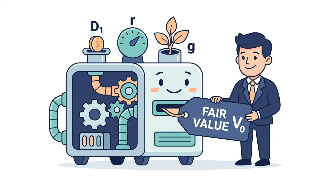
The Gordon Growth Model values a dividend stock from one fraction: V₀ = D₁ / (r − g). Three inputs, no calculus. It is the simplest form of the dividend discount model and the same formula provides the terminal value inside almost every DCF model. The interesting input is g, and the textbook derivation is g = retention ratio × ROE.
Our DCF calculator lets you tie the Gordon assumption back into a full cash-flow model.
The Gordon Growth Formula
The formula is one line:
V₀ is the fair value per share today. D₁ is the expected dividend one year from now. r is the required rate of return. g is the constant rate at which dividends grow forever.
The intuition is an infinite geometric series collapsed into a fraction. Dividends grow at g each year and get discounted back at r, so a single subtraction in the denominator does all the work.
One rule cannot bend: r must exceed g. When g catches up to r, the denominator hits zero and the valuation explodes toward infinity, which is the model's way of saying the assumption is wrong.
Sustainable Growth: g = Retention × ROE
The hardest input to pick is g. The cleanest derivation is the sustainable growth rate:
b is the retention ratio: one minus the dividend payout ratio. ROE is return on equity. The intuition is mechanical: retained earnings reinvested at the firm's ROE compound at exactly that rate.
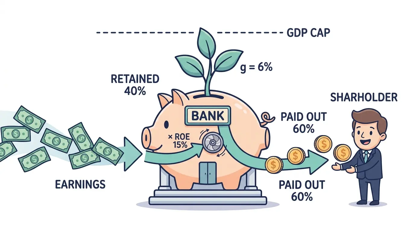
Worked example. A consumer staples firm earns a 15% ROE and keeps 40% of profits (payout ratio 60%). The implied sustainable growth rate is:
Plug 6% back into Gordon for the fair-value calculation in the next section.
The GDP cap. Aswath Damodaran's rule: g cannot exceed long-run nominal GDP growth, since no firm outgrows its own economy forever. For developed markets that ceiling sits near 4% to 5%. If retention × ROE produces 12%, the cap binds and the input becomes the cap, not the raw derivation.
Where the derivation breaks. Cyclical companies have unstable ROE: the formula gives nonsense in a recession. Firms returning cash through share buybacks violate the assumption that retention reinvests cleanly. Use the derivation for mature, dividend-paying, profitable firms with steady reinvestment patterns.
Choosing r and D₁
Two more inputs, both lighter than g.
D₁: next year's expected dividend. Most analysts start from the last dividend paid and grow it by one year: D₁ = D₀ × (1 + g). A $2.00 dividend with 5% growth gives D₁ = $2.10.
r: the required return. The CAPM build is the risk-free rate plus beta times the equity risk premium. The WACC calculator gives a defensible starting point for the cost of equity. In practice many investors use a hurdle rate in the 8% to 12% range.
The interaction between r and g matters more than either input alone. A 5-point spread produces stable valuations. A 1-point spread produces numbers that swing wildly on any input change, which the next section quantifies.
A Worked Example and the Sensitivity That Bites
Take a mature consumer staples firm. Next year's dividend is $2.00, the required return is 8%, and dividends have grown at 4% for the last decade.
At $45 the model calls it undervalued. At $58, overvalued.
Now move one input. Push g from 4% to 5%:
A single percentage point on growth added 33% to the fair value. Push r to 9% instead and the answer drops to $40. The sensitivity table for a $2.00 dividend across different r minus g spreads:
| r − g spread | Fair value |
|---|---|
| 5% | $40.00 |
| 4% | $50.00 |
| 3% | $66.67 |
| 2% | $100.00 |
| 1% | $200.00 |
Every point the spread narrows roughly doubles the valuation. Most analysts run a sensitivity grid rather than report a single number. The math is clean. The output is only as stable as the weakest input.
Terminal Value: Gordon Inside Every DCF
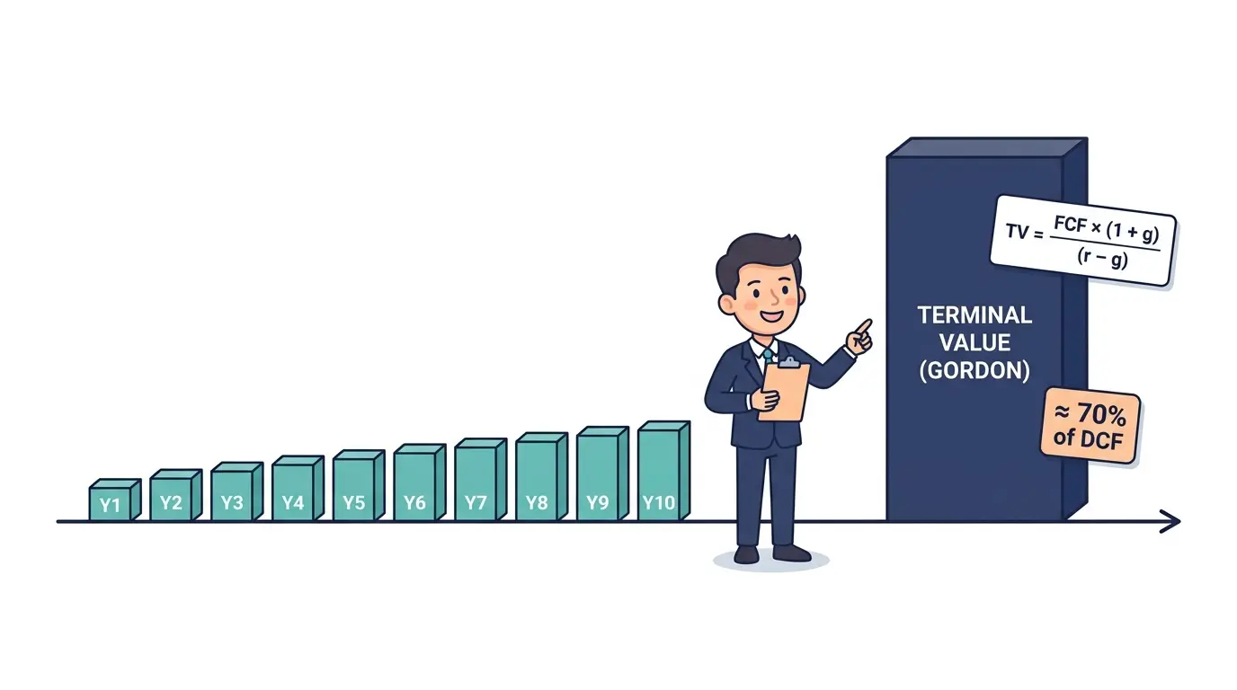
Most professionals never value a whole stock with pure Gordon Growth. They use it for the tail of something bigger. Inside a discounted cash flow model, analysts project free cash flows explicitly for 5 or 10 years, then switch to a terminal value for everything after. The standard terminal value formula is Gordon dressed up for cash flow:
That single line often represents 60% to 80% of the DCF total, so the Gordon assumption does most of the work in cash-flow-based models. The discipline is to test the sensitivity of TV to small changes in g and WACC before treating the DCF output as a point estimate.
The same structure values the broad market: plug the S&P 500 forward dividend into D₁, the equity risk premium plus the risk-free rate into r, and long-run GDP growth into g.
Where the Model Breaks
The model fails quietly for most of the modern equity market. Growth companies that pay no dividend have no D₁, so there is nothing to discount. Cyclicals have real earnings but no steady g to plug in.
Other failure modes are subtler.
g approaching r: As the denominator shrinks, the valuation becomes theater. Any firm with expected growth close to its cost of equity needs a multi-stage model or a reverse DCF that solves for the growth the market is already pricing in.
Payout changes: A company that cuts its dividend in a recession breaks every Gordon projection retroactively, no matter how defensible the prior inputs looked.
Ignored optionality: Brand value, reinvestment returns, and buyback capacity sit outside the equation.
Use the formula where its assumptions hold: mature dividend payers, regulated utilities, and index-level valuations. Screen candidates on the dividend yield heatmap, check that the r minus g spread sits comfortably wide, and run the DCF calculator to put the Gordon assumption inside a full cash-flow model before trusting any single number.
Frequently Asked Questions
What is the formula for the Gordon Growth Model? The Gordon Growth Model formula is V₀ = D₁ / (r − g). V₀ is the fair value per share today. D₁ is the dividend expected one year from now. r is the required rate of return, usually the cost of equity. g is the long-run dividend growth rate. The formula collapses an infinite stream of growing dividends into one fraction.
How is g calculated from retention ratio and ROE? The standard derivation is g = retention ratio × ROE. The retention ratio is one minus the dividend payout ratio. A company earning 15% ROE that retains 40% of profits has an implied sustainable growth rate of 6%. Retained earnings reinvested at the firm's ROE compound at exactly that rate. Cap the result at long-run nominal GDP growth, since no firm outgrows its own economy indefinitely.
Is the Gordon Growth Model a DCF? Yes, in the strict sense. Both discount future cash flows back to present value. The Gordon Growth Model is the simplest dividend-based DCF: it assumes one constant growth rate forever, so the infinite sum collapses to D₁ / (r − g). A full DCF projects free cash flows explicitly for several years before switching to a Gordon-style terminal value for the tail.
Is the Gordon Growth Model the same as the Dividend Discount Model? The Gordon Growth Model is the constant-growth version of the dividend discount model, and the version most people mean when they say DDM. It assumes one growth rate forever. Multi-stage DDMs let growth shift over time at the cost of extra inputs and more assumptions to defend.